OVERVIEW

In this assignment, we are going to practice creating visualizations for tabular data. Unlike previous assignments, however, this time we will all be using the same data sets. I’m doing this because I want everyone to engage in the same logic process and have the same design objectives in mind.

LEARNING OBJECTIVES

Demonstrate that you can manipulate tabular data to facilitate different visualization tasks. The minimum skills are FILTERING, SELECTING, and SUMMARIZING, all while GROUPING these operations as dictated by your data.
Demonstrate that you can use tabular data to explore, analyze, and choose the most appropriate visualization idioms given a specific motivating question.
Demonstrate that you can Find, Access, and Integrate additional data in order to fully address the motivating question.

The scenario below will allow you to complete the assignment. It deals with data that are of the appropriate complexity and extent (number of observations and variables) to challenge you. If you want to use different data (yours or from another source) I am happy to work with you to make that happen!

SCENARIO

We are going to use NHL data on the season to date to create data driven ballots for several key awards. The awards we will consider are:

Hart Memorial Trophy

Awarded to the “player judged most valuable to his team.” This isn’t necessarily the best overall player, but rather the one who contributes most significantly to his team’s success.

Vezina Trophy

Presented to the goaltender “adjudged to be the best at this position.” NHL general managers vote on this award.

James Norris Memorial Trophy

Awarded to the defenseman who demonstrates “the greatest all-around ability” at the position.

Calder Memorial Trophy

Given to the player “adjudged to be the most proficient in his first year of competition.” This is essentially the rookie of the year award.

Frank J. Selke Trophy

Awarded to the forward who best excels in the defensive aspects of the game.

Lady Byng Memorial Trophy

Presented to the player who exhibits “the best type of sportsmanship and gentlemanly conduct combined with a high standard of playing ability.”

Note that I’ve eliminated the awards that are determined by raw counting statistics (most goals, most points). The awards above are all based on votes from NHL media and executives, and the criteria are at least somewhat subjective.

Here is the goal:

For each award, create your ballot of five players, ranked from 1 (your first choice) to 5 (your fifth choice). For each ballot, provide one to three visualizations that explain and justify your ballot.

DIRECTIONS

Create a new post in your portfolio for this assignment. Call it something cool, like NHL player award analysis, or Hockey Analytics, or John Wick….

Copy the data files from the repository, and maybe also the .qmd file.

Use the .qmd file as the backbone of your assignment, changing the code and the markdown text as you go.

THE DATA

At minimum, we will use the data from naturalstattrick.com for player statistics for the season to date (Oct 2024 to March 2025). You can find the Data Dictionary here

Code

Indivdual.Skater <- read.csv("SkaterIndividualstats.csv")
OnIce.Skater <- read.csv("SkaterOnicestats.csv")
Goalie <- read.csv("Goalies.csv")
Individual.Skater.Rookie <- read.csv("RookieSkaterindividual.csv")
OnIce.Skater.Rookie <- read.csv("RookieSkaterOnIce.csv")
Rookie.Goalie <- read.csv("RookieGoalies.csv")

This code reads in the data files into dataframes. You will have to decide which dataframes correspond to which awards. Some awards will be informed by more than one dataframe.

HOW TO GET STARTED

There is a lot of data here, and you probably don’t need all of it. The counting stats that you should start with are pretty simple. For skaters, it is Total Points, which is the sum of Goals and Assists. Assists can be primary (the person who made the pass to the scorer) or secondary (the person who made the pass to the primary assist player), but I wouldn’t worry about that for now. For goaltenders, it is save percentage and goals against average.

HOWEVER, counting stats don’t tell the whole story in hockey. Hockey is a low event sport, so goals are somewhat rare. This is where the advanced stats come in to play. These are usually found in the “OnIce” data sets. Here, I’d start with Corsi Statistics and Expected Goals Statistics, which are defined below.

Corsi Statistics

Corsi: Any shot attempt (goals, shots on net, misses and blocks) outside of the shootout. Referred to as SAT by the NHL.

Term	Definition
CF	Count of Corsi for that player’s team while that player is on the ice.
CA	Count of Corsi against that player’s team while that player is on the ice.
CF%	Percentage of total Corsi while that player is on the ice that are for that player’s team. CF*100/(CF+CA)

Expected Goals

Expected goals (xG) is a statistical measure that evaluates shot quality by assigning a goal probability to each shot attempt.

Term	Definition
xGF	Expected Goals For. The sum of the probability values of all shot attempts for that player’s team while that player is on the ice. Represents the number of goals the team should have scored based on shot quality.
xGA	Expected Goals Against. The sum of the probability values of all shot attempts against that player’s team while that player is on the ice. Represents the number of goals the team should have conceded based on shot quality.
xGF%	Expected Goals Percentage. The percentage of the total expected goals while that player is on the ice that are for that player’s team. xGF*100/(xGF+xGA)

Let’s have a look at the distributions of some of these stats!

Counting Stats for Skaters

Code

ggplot(Indivdual.Skater, aes(x=Total.Points))+
  geom_histogram(binwidth = 1)+
  labs(x = "Total Points",
       y = "Number of Players",
       caption = "source: https://www.naturalstattrick.com/",
       title = "Distribution of Total Points",
       subtitle = "2024-2025 season stats as of March 4")

Code

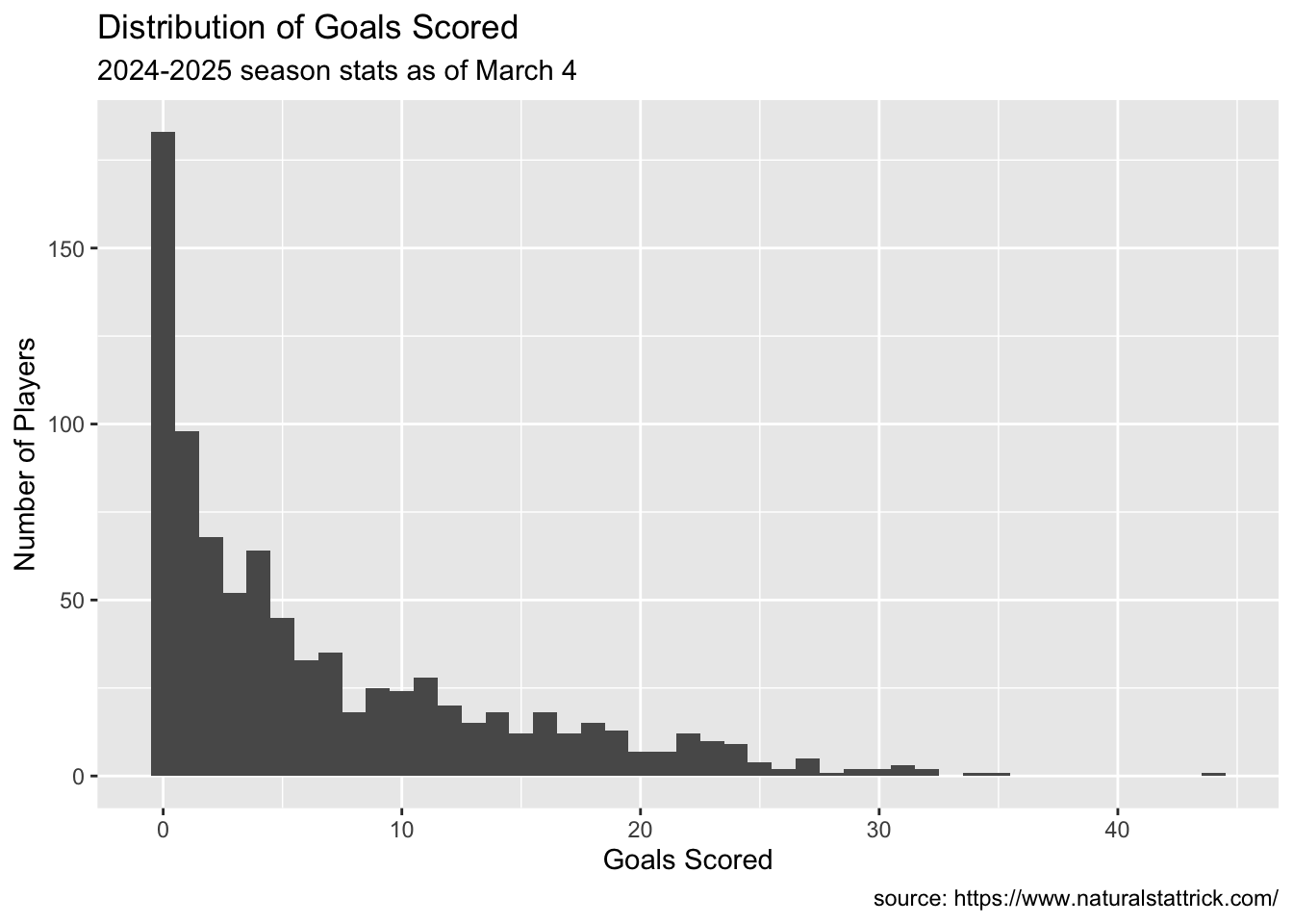
ggplot(Indivdual.Skater, aes(x=Goals))+
  geom_histogram(binwidth = 1)+
  labs(x = "Goals Scored",
       y = "Number of Players",
       caption = "source: https://www.naturalstattrick.com/",
       title = "Distribution of Goals Scored",
       subtitle = "2024-2025 season stats as of March 4")

Code

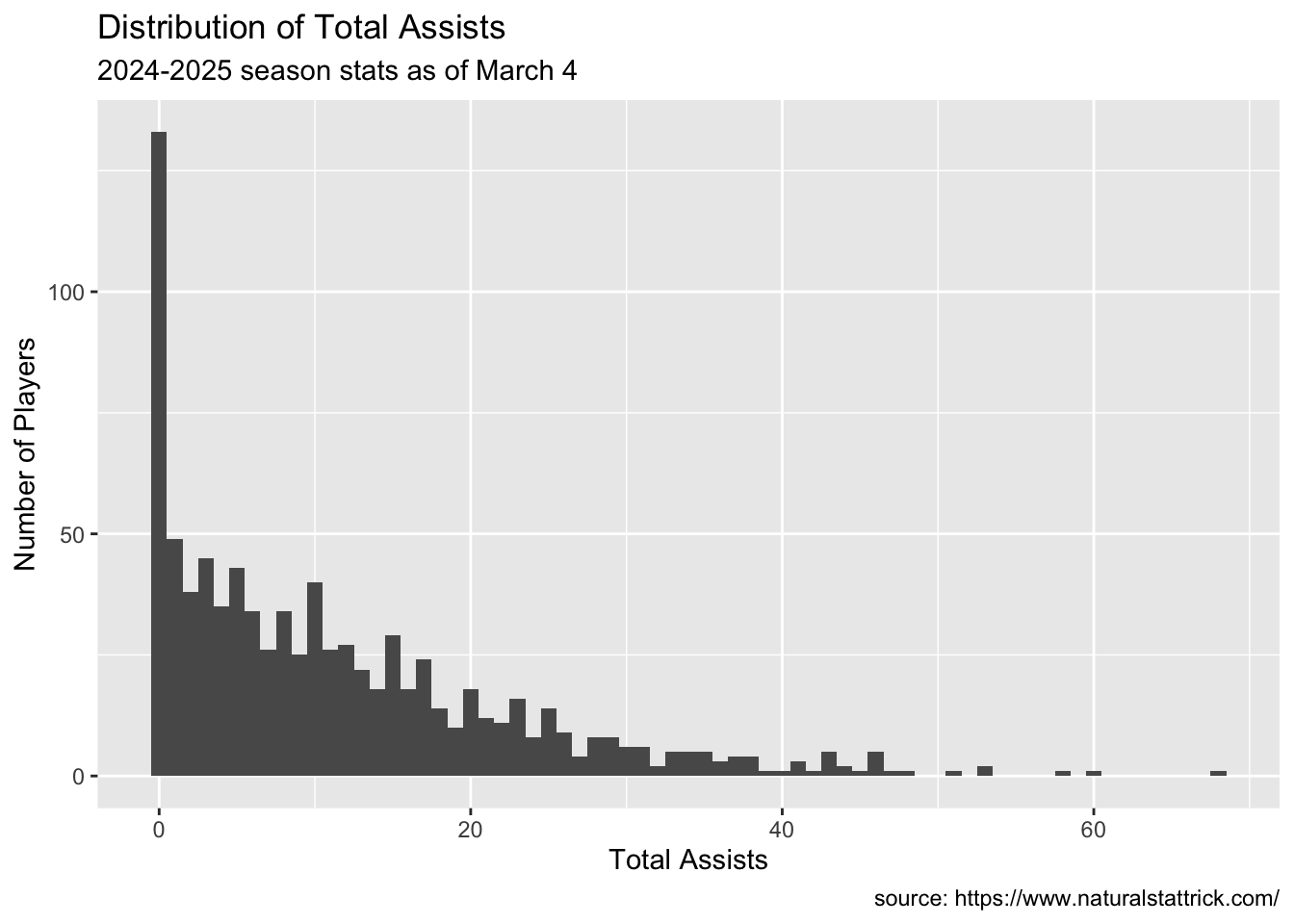
ggplot(Indivdual.Skater, aes(x=Total.Assists))+
  geom_histogram(binwidth = 1)+
  labs(x = "Total Assists",
       y = "Number of Players",
       caption = "source: https://www.naturalstattrick.com/",
       title = "Distribution of Total Assists",
       subtitle = "2024-2025 season stats as of March 4")

On Ice Stats for Skaters

Code

ggplot(OnIce.Skater, aes(x=CF.))+
  geom_histogram(binwidth = 1)+
  labs(x = "Corsi Percentage",
       y = "Number of Players",
       caption = "source: https://www.naturalstattrick.com/",
       title = "Distribution of Corsi Percentage",
       subtitle = "2024-2025 season stats as of March 4")

Code

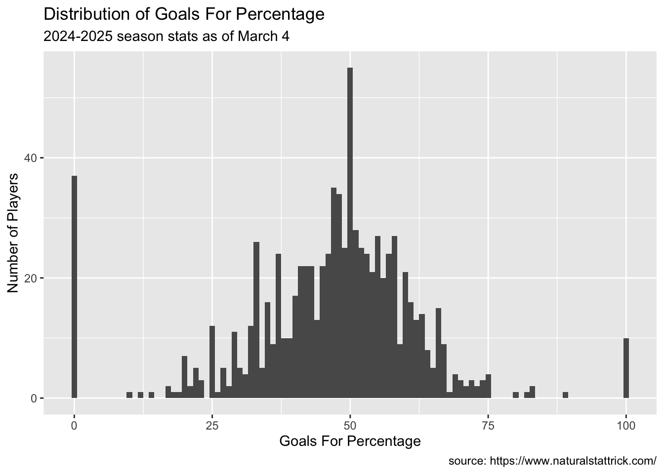
ggplot(OnIce.Skater, aes(x=as.numeric(GF.)))+
  geom_histogram(binwidth = 1)+
  labs(x = "Goals For Percentage",
       y = "Number of Players",
       caption = "source: https://www.naturalstattrick.com/",
       title = "Distribution of Goals For Percentage",
       subtitle = "2024-2025 season stats as of March 4")

Warning in FUN(X[[i]], ...): NAs introduced by coercion

Warning: Removed 18 rows containing non-finite outside the scale range
(`stat_bin()`).

Code

ggplot(OnIce.Skater, aes(x=as.numeric(xGF.)))+
  geom_histogram(binwidth = 1)+
  labs(x = "Expected Goals For Percentage",
       y = "Number of Players",
       caption = "source: https://www.naturalstattrick.com/",
       title = "Distribution of Expected Goals For Percentage",
       subtitle = "2024-2025 season stats as of March 4")

Stats for Goalies

Code

ggplot(Goalie, aes(x=SV.))+
  geom_histogram(binwidth = .01)+
  labs(x = "Save Percentage",
       y = "Number of Players",
       caption = "source: https://www.naturalstattrick.com/",
       title = "Distribution of Save Percentage",
       subtitle = "2024-2025 season stats as of March 4")

Code

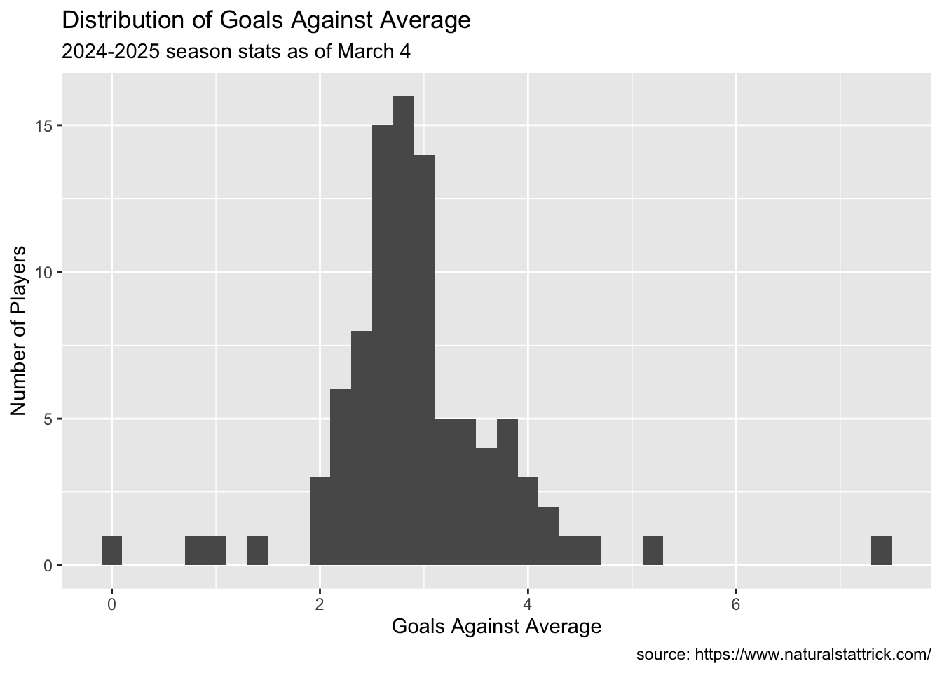
ggplot(Goalie, aes(x=GAA))+
  geom_histogram(binwidth = .2)+
  labs(x = "Goals Against Average",
       y = "Number of Players",
       caption = "source: https://www.naturalstattrick.com/",
       title = "Distribution of Goals Against Average",
       subtitle = "2024-2025 season stats as of March 4")

Code

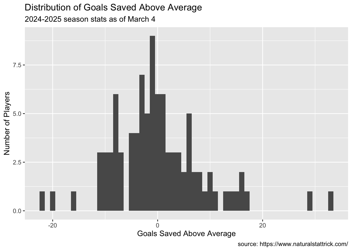
ggplot(Goalie, aes(x=GSAA))+
  geom_histogram(binwidth = 1)+
  labs(x = "Goals Saved Above Average",
       y = "Number of Players",
       caption = "source: https://www.naturalstattrick.com/",
       title = "Distribution of Goals Saved Above Average",
       subtitle = "2024-2025 season stats as of March 4")

Of all of the awards above, the easiest one to start with is the Vezina Trophy, which is presented to the goaltender “adjudged to be the best at this position.” NHL general managers vote on this award, but its pretty easy to use goaltending stats to inform your vote.

Think about how our task maps on to our data. What are we trying to do here? What visual channels are best used to accomplish the task?

THE TIDYVERSE

I’m using the Tidyverse to manipulate my data. I set up the original data frame to conform to the tidy data principles (every column is a variable, every row is an observation), which is pretty much the base form of how we’ve discussed Tabular Data in class.

You are likely to use the functions that FILTER, GROUP, and SUMMARIZE the data, often creating new dataframes for downstream analysis or visualization. Hey, look! A handy cheatsheet for data transformation using the tidyverse!

These functions come from the dplyr package that gets installed as part of the tidyverse. The basic categories of actions are:

mutate() adds new variables that are functions of existing variables
select() picks variables based on their names.
filter() picks cases based on their values.
summarise() reduces multiple values down to a single summary.
arrange() changes the ordering of the rows.

All of these work with group_by() so you can perform whichever operation on the groups that might be present in your data set.

--- title: "ASSIGNMENT 5" subtitle: "Visualizations for Tabular Data" author: "Barrie Robison" date: "2025-02-27" categories: [Assignment, DataViz, Tables, Scatterplot, Barplot, Piechart] image: "Cthulhuhockeycard.png" code-fold: true code-tools: true description: "Data driven voting for NHL awards" --- # OVERVIEW In this assignment, we are going to practice creating visualizations for tabular data. Unlike previous assignments, however, this time we will all be using the same data sets. I'm doing this because I want everyone to engage in the same logic process and have the same design objectives in mind. # LEARNING OBJECTIVES 1. Demonstrate that you can manipulate tabular data to facilitate different visualization tasks. The minimum skills are FILTERING, SELECTING, and SUMMARIZING, all while GROUPING these operations as dictated by your data. 2. Demonstrate that you can use tabular data to explore, analyze, and choose the most appropriate visualization idioms given a specific motivating question. 3. Demonstrate that you can Find, Access, and Integrate additional data in order to fully address the motivating question. The scenario below will allow you to complete the assignment. It deals with data that are of the appropriate complexity and extent (number of observations and variables) to challenge you. If you want to use different data (yours or from another source) I am happy to work with you to make that happen! # SCENARIO We are going to use NHL data on the season to date to create data driven ballots for several key awards. The awards we will consider are: ## Hart Memorial Trophy Awarded to the "player judged most valuable to his team." This isn't necessarily the best overall player, but rather the one who contributes most significantly to his team's success. ## Vezina Trophy Presented to the goaltender "adjudged to be the best at this position." NHL general managers vote on this award. ## James Norris Memorial Trophy Awarded to the defenseman who demonstrates "the greatest all-around ability" at the position. ## Calder Memorial Trophy Given to the player "adjudged to be the most proficient in his first year of competition." This is essentially the rookie of the year award. ## Frank J. Selke Trophy Awarded to the forward who best excels in the defensive aspects of the game. ## Lady Byng Memorial Trophy Presented to the player who exhibits "the best type of sportsmanship and gentlemanly conduct combined with a high standard of playing ability." Note that I've eliminated the awards that are determined by raw counting statistics (most goals, most points). The awards above are all based on votes from NHL media and executives, and the criteria are at least somewhat subjective. ### Here is the goal: For each award, create your ballot of five players, ranked from 1 (your first choice) to 5 (your fifth choice). For each ballot, provide one to three visualizations that explain and justify your ballot. ## DIRECTIONS Create a new post in your portfolio for this assignment. Call it something cool, like NHL player award analysis, or Hockey Analytics, or John Wick.... Copy the data files from the repository, and maybe also the .qmd file. Use the .qmd file as the backbone of your assignment, changing the code and the markdown text as you go. ## THE DATA At minimum, we will use the data from naturalstattrick.com for player statistics for the season to date (Oct 2024 to March 2025). You can find the Data Dictionary [here](DataDictionary.qmd) ```{r include=FALSE} library(tidyverse) library(readxl) ``` ```{r} Indivdual.Skater <- read.csv("SkaterIndividualstats.csv") OnIce.Skater <- read.csv("SkaterOnicestats.csv") Goalie <- read.csv("Goalies.csv") Individual.Skater.Rookie <- read.csv("RookieSkaterindividual.csv") OnIce.Skater.Rookie <- read.csv("RookieSkaterOnIce.csv") Rookie.Goalie <- read.csv("RookieGoalies.csv") ``` This code reads in the data files into dataframes. You will have to decide which dataframes correspond to which awards. Some awards will be informed by more than one dataframe. ## HOW TO GET STARTED There is a lot of data here, and you probably don't need all of it. The counting stats that you should start with are pretty simple. For skaters, it is Total Points, which is the sum of Goals and Assists. Assists can be primary (the person who made the pass to the scorer) or secondary (the person who made the pass to the primary assist player), but I wouldn't worry about that for now. For goaltenders, it is save percentage and goals against average. [HOWEVER]{.red}, counting stats don't tell the whole story in hockey. Hockey is a low event sport, so goals are somewhat rare. This is where the advanced stats come in to play. These are usually found in the "OnIce" data sets. Here, I'd start with **Corsi Statistics** and **Expected Goals Statistics**, which are defined below. ### Corsi Statistics **Corsi**: Any shot attempt (goals, shots on net, misses and blocks) outside of the shootout. Referred to as SAT by the NHL. | Term | Definition | |------|------------| | **CF** | Count of Corsi for that player's team while that player is on the ice. | | **CA** | Count of Corsi against that player's team while that player is on the ice. | | **CF%** | Percentage of total Corsi while that player is on the ice that are for that player's team. CF*100/(CF+CA) | ### Expected Goals Expected goals (xG) is a statistical measure that evaluates shot quality by assigning a goal probability to each shot attempt. | Term | Definition | |------|------------| | **xGF** | Expected Goals For. The sum of the probability values of all shot attempts for that player's team while that player is on the ice. Represents the number of goals the team should have scored based on shot quality. | | **xGA** | Expected Goals Against. The sum of the probability values of all shot attempts against that player's team while that player is on the ice. Represents the number of goals the team should have conceded based on shot quality. | | **xGF%** | Expected Goals Percentage. The percentage of the total expected goals while that player is on the ice that are for that player's team. xGF*100/(xGF+xGA) | Let's have a look at the distributions of some of these stats! ## Counting Stats for Skaters ```{r} ggplot(Indivdual.Skater, aes(x=Total.Points))+ geom_histogram(binwidth = 1)+ labs(x = "Total Points", y = "Number of Players", caption = "source: https://www.naturalstattrick.com/", title = "Distribution of Total Points", subtitle = "2024-2025 season stats as of March 4") ggplot(Indivdual.Skater, aes(x=Goals))+ geom_histogram(binwidth = 1)+ labs(x = "Goals Scored", y = "Number of Players", caption = "source: https://www.naturalstattrick.com/", title = "Distribution of Goals Scored", subtitle = "2024-2025 season stats as of March 4") ggplot(Indivdual.Skater, aes(x=Total.Assists))+ geom_histogram(binwidth = 1)+ labs(x = "Total Assists", y = "Number of Players", caption = "source: https://www.naturalstattrick.com/", title = "Distribution of Total Assists", subtitle = "2024-2025 season stats as of March 4") ``` ## On Ice Stats for Skaters ```{r} ggplot(OnIce.Skater, aes(x=CF.))+ geom_histogram(binwidth = 1)+ labs(x = "Corsi Percentage", y = "Number of Players", caption = "source: https://www.naturalstattrick.com/", title = "Distribution of Corsi Percentage", subtitle = "2024-2025 season stats as of March 4") ggplot(OnIce.Skater, aes(x=as.numeric(GF.)))+ geom_histogram(binwidth = 1)+ labs(x = "Goals For Percentage", y = "Number of Players", caption = "source: https://www.naturalstattrick.com/", title = "Distribution of Goals For Percentage", subtitle = "2024-2025 season stats as of March 4") ggplot(OnIce.Skater, aes(x=as.numeric(xGF.)))+ geom_histogram(binwidth = 1)+ labs(x = "Expected Goals For Percentage", y = "Number of Players", caption = "source: https://www.naturalstattrick.com/", title = "Distribution of Expected Goals For Percentage", subtitle = "2024-2025 season stats as of March 4") ``` ## Stats for Goalies ```{r} ggplot(Goalie, aes(x=SV.))+ geom_histogram(binwidth = .01)+ labs(x = "Save Percentage", y = "Number of Players", caption = "source: https://www.naturalstattrick.com/", title = "Distribution of Save Percentage", subtitle = "2024-2025 season stats as of March 4") ggplot(Goalie, aes(x=GAA))+ geom_histogram(binwidth = .2)+ labs(x = "Goals Against Average", y = "Number of Players", caption = "source: https://www.naturalstattrick.com/", title = "Distribution of Goals Against Average", subtitle = "2024-2025 season stats as of March 4") ggplot(Goalie, aes(x=GSAA))+ geom_histogram(binwidth = 1)+ labs(x = "Goals Saved Above Average", y = "Number of Players", caption = "source: https://www.naturalstattrick.com/", title = "Distribution of Goals Saved Above Average", subtitle = "2024-2025 season stats as of March 4") ``` Of all of the awards above, the easiest one to start with is the **Vezina Trophy**, which is presented to the goaltender "adjudged to be the best at this position." NHL general managers vote on this award, but its pretty easy to use goaltending stats to inform your vote. Think about how our task maps on to our data. What are we trying to do here? What visual channels are best used to accomplish the task? ## THE TIDYVERSE I'm using the [Tidyverse](https://www.tidyverse.org) to manipulate my data. I set up the original data frame to conform to the tidy data principles (every column is a variable, every row is an observation), which is pretty much the base form of how we've discussed [Tabular Data](../L6-TabularData1) in class. You are likely to use the functions that FILTER, GROUP, and SUMMARIZE the data, often creating new dataframes for downstream analysis or visualization. Hey, look! [A handy cheatsheet for data transformation using the tidyverse!](https://github.com/rstudio/cheatsheets/blob/main/data-transformation.pdf) These functions come from the [dplyr package](https://dplyr.tidyverse.org) that gets installed as part of the tidyverse. The basic categories of actions are: - mutate() adds new variables that are functions of existing variables - select() picks variables based on their names. - filter() picks cases based on their values. - summarise() reduces multiple values down to a single summary. - arrange() changes the ordering of the rows. All of these work with group_by() so you can perform whichever operation on the groups that might be present in your data set.