TUTORIAL 2 - Literate Programming and Anscombe’s Quartet

MORE QUARTO!

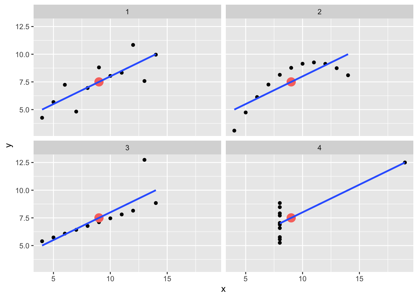
Do the summary statistics reveal the truth? Or are they FILLED WITH LIES? A simple demonstration with Anscombe’s Quartet.

Again, the video is a couple years old. Expect a few dated references.

ANSCOMBE’S QUARTET

The purpose of this assignment is to demonstrate how summary statistics can sometimes be misleading and how data visualization helps us understand our dataset.

The Data

Anscombe’s Quartet is comprised of four pairs of x,y data:

library(ggplot2)
library(grid)
library(gridExtra)
library(datasets)
library(tidyverse)
library(dplyr)

datasets::anscombe

   x1 x2 x3 x4    y1   y2    y3    y4
1  10 10 10  8  8.04 9.14  7.46  6.58
2   8  8  8  8  6.95 8.14  6.77  5.76
3  13 13 13  8  7.58 8.74 12.74  7.71
4   9  9  9  8  8.81 8.77  7.11  8.84
5  11 11 11  8  8.33 9.26  7.81  8.47
6  14 14 14  8  9.96 8.10  8.84  7.04
7   6  6  6  8  7.24 6.13  6.08  5.25
8   4  4  4 19  4.26 3.10  5.39 12.50
9  12 12 12  8 10.84 9.13  8.15  5.56
10  7  7  7  8  4.82 7.26  6.42  7.91
11  5  5  5  8  5.68 4.74  5.73  6.89

Example Hypotheses

1. Betsy has four replicates in which she is measuring the abundance of two bacteria (x, y) on 11 milk samples.
2. Priya has four replicates in which she is measuring gene expression of two genes (x, y) in 11 different pipefish tissue samples.
3. Henry has four replicate years in which he is measuring the abundance of an insect pest (x) and crop productivity (y) in 11 fields.

Your hypothesis is that the four replicates do not differ in the correlation between x and y.

Summary Statistics

tidy_anscombe <- anscombe %>%
 pivot_longer(cols = everything(),
              names_to = c(".value", "set"),
              names_pattern = "(.)(.)")
tidy_anscombe_summary <- tidy_anscombe %>%
  group_by(set) %>%
  summarise(across(.cols = everything(),
                   .fns = lst(min,max,median,mean,sd,var),
                   .names = "{col}_{fn}"))
#> `summarise()` ungrouping output (override with `.groups` argument)

vars<-c("set", "x_mean", "x_var",  "y_mean", "y_var")
thing<- as.data.frame(tidy_anscombe_summary[vars])
knitr::kable(thing)

set	x_mean	x_var	y_mean	y_var
1	9	11	7.500909	4.127269
2	9	11	7.500909	4.127629
3	9	11	7.500000	4.122620
4	9	11	7.500909	4.123249

Visualization reveals hidden patterns!

ggplot(tidy_anscombe,
       aes(x = x,
           y = y)) +
  geom_point() +
  geom_point(data = tidy_anscombe_summary, aes(x=x_mean, y = y_mean, color = "red", size = 5),
             show.legend = FALSE)+
  facet_wrap(~set) +
  geom_smooth(method = "lm", se = FALSE)

`geom_smooth()` using formula = 'y ~ x'